Enhanced Estimator
enhanced.Rmd
library(XSRecency)In this vignette, we show how to use the enhanced estimator that incorporates prior HIV test results into the cross-sectional incidence estimate. In the process, we will show how to use the data to estimate properties of recent infection testing algorithms.
Estimate a phi function based on a recent infection testing algorithm from data
Define algorithm of recent infection, and obtain data
Can either use the pre-loaded data in this package, or use your own
that you have downloaded through the function with the optional argument
filepath.
# Define a recent infection as LAg <= 1.5 and viral load > 1000
f <- function(l, v){
 v <- ifelse(l > 1.5, 0, v)
 return(
   ifelse((l <= 1.5) & (v > 1000), 1, 0)
 )
}

# Get dataset
phidat <- createRitaCephia(assays=c("LAg-Sedia", "viral_load"), algorithm=f)
#> There are 53 missing values for viral_load
#> Removing 10 observations with missing recency indicator after application of the algorithm.

# Convert infection duration to years
phidat$ui <- phidat$ui / 365.25
head(phidat)
#>          id        ui ri
#> 1: 72748497 1.9603012  0
#> 2: 72748497 2.4202601  0
#> 3: 87007074 0.9856263  0
#> 4: 87007074 1.9055441  0
#> 5: 87007074 3.2580424  0
#> 6: 44656860 1.0047912  0
Estimate test-recent function
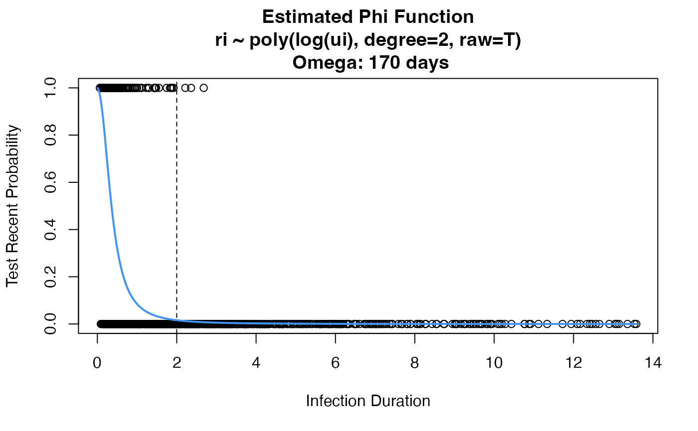
We can now use the CEPHIA data from above to estimate a phi function. We are doing this purely for the purposes of simulation. Usually, this is done internally in the function.
# use this argument if you want to get an estimated phi function, rather than just MDRI summary
rita.props <- estRitaProperties(
  phidat=phidat,
  maxT=10,
  bigT=2,
  use_geese=TRUE, # need this when have multiple observations per individual
  formula="ri ~ poly(log(ui), degree=2, raw=T)",
  family=binomial(link="logit"),
  min_dt=TRUE, # need this when doing log(ui)
  return_all=T,
  plot_phi=T
)
Simulate cross-sectional incidence data and prior HIV testing data
Cross-sectional incidence data
# Use our estimated phi function to simulate recent infection indicators
sim <- simCrossSect(phi.func=rita.props$phi,
                    incidence_type="constant", prevalence=0.29, baseline_incidence=0.032)
set.seed(10)
df <- sim(5000)
Prior HIV testing data
Simulate prior HIV tests as 10% of HIV positive individuals having uniformly distributed tests over the last 4 years
sim.pt <- simPriorTests(ptest.dist=function(u) runif(1, 0, 4),
                        ptest.prob=function(u) 0.1)

# Create prior testing data frame, only for those who are positive
ptdf <- sim.pt(df[df$di == 1,])
head(ptdf)
#>      di        ui ri ti qi deltai
#> 3524  1  3.309033  0 NA  0     NA
#> 3525  1  3.470821  0 NA  0     NA
#> 3526  1  4.790286  0 NA  0     NA
#> 3527  1 10.650930  0 NA  0     NA
#> 3528  1  9.697202  0 NA  0     NA
#> 3529  1 11.150070  0 NA  0     NA
Apply Enhanced Estimator
Apply the enhanced estimator using the CEPHIA data before that we used to simulate our current dataset, and the same model for the test-recent function. See for details on additional values returned.
estimate <- estEnhanced(
  n_p=nrow(ptdf),
  n=nrow(df),
  ptdf=ptdf,
  beta=0,
  beta_var=0,
  big_T=2,
  phidat=phidat,
  use_geese=TRUE,
  formula="ri ~ poly(log(ui), degree=2, raw=T)",
  family=binomial(link="logit"),
  min_dt=TRUE
)

estimate$est
#> [1] 0.0329671
estimate$var
#> [1] 2.043809e-05